
The Impact of Decision Threshold Optimization
Fine-Tune Decision Points for Better Model Results

Introduction
The decision threshold is a critical yet frequently overlooked hyperparameter in binary classification tasks. It dictates the cutoff point at which a model assigns a data point to one of two classes. Typically, machine learning algorithms default to a threshold of 0.5, classifying a data point as positive if its predicted probability meets or exceeds this value. However, this default setting may not be optimal for every scenario. In this article, we'll explore how adjusting the decision threshold can significantly impact model performance, using a simple synthetic data study in Python to illustrate the concept.
The Synthetic Dataset
We start by generating a synthetic dataset with a linear combination of two variables and some noise. This dataset contains a defined imbalance ratio, which means we control the proportion of positive and negative classes. In our case, we've set an imbalance ratio of 0.2, which results in 80% of the data being in the negative class and 20% in the positive class. You can play with this ratio to see how it affects the threshold optimization process.
import numpy as np
import pandas as pd
from sklearn.model_selection import train_test_split
from sklearn.linear_model import LogisticRegression
import matplotlib.pyplot as plt

# Generate synthetic data with a linear combination of two variables and noise
np.random.seed(0)
n_samples = 100000
X1 = np.random.randn(n_samples)
X2 = 2 * X1 + np.random.normal(0, 1, n_samples)

# Feel free to play with the noise here. Less noise, even with imbalanced data, will allow the model to discriminate better.
# Therefore changing the default threshold away from 0.5 won't matter as much
noise = np.random.normal(0, 1.5, n_samples)

# Set the desired imbalance ratio (e.g., 90% negative class, 10% positive class)
imbalance_ratio = 0.2 # <--- Feel free to play with the imbalance here
threshold = np.percentile(0.7 * X1 + 0.3 * X2 + noise, 100 * (1 - imbalance_ratio))
y = (0.7 * X1 + 0.3 * X2 + noise > threshold).astype(int)

# Split the dataset into training and testing sets
X = np.column_stack((X1, X2))
X_train, X_test, y_train, y_test = train_test_split(X, y, test_size=0.2, random_state=42)
Training a Logistic Regression Model
We then split our dataset into training and testing sets and train a logistic regression model. Note that in a real world scenario, you should also have an additional test set of data that is completely held out and only used to make a final evaluation of the model. No updates to the model or hyperparameters should be done based on the results generated from the held-out test set, otherwise you risk overfitting the model and won’t get an unbiased estimate of the model’s performance.
Now onto the simple toy model. The logistic regression model is a simple yet effective classifier that assigns probabilities to each data point. These probabilities can be used to calculate various performance metrics.
# Fit a logistic regression model
model = LogisticRegression()
model.fit(X_train, y_train)

# Predicted probabilities
predicted_probabilities = model.predict_proba(X_test)[:, 1]

# Plot the predicted probabilities
plt.figure(figsize=(10, 6))
plt.hist(predicted_probabilities[y_test == 1], bins=100, alpha=0.5, color='blue', label='Positive Class (1)')
plt.hist(predicted_probabilities[y_test == 0], bins=100, alpha=0.5, color='red', label='Negative Class (0)')
plt.xlabel('Predicted Probabilities')
plt.ylabel('Frequency')
plt.legend(loc='best')
plt.title('Predicted Probabilities for an Imbalanced Dataset (Custom Imbalance Ratio)')
plt.xlim(0, 1)  # Set the x-axis limits between 0 and 1
plt.show()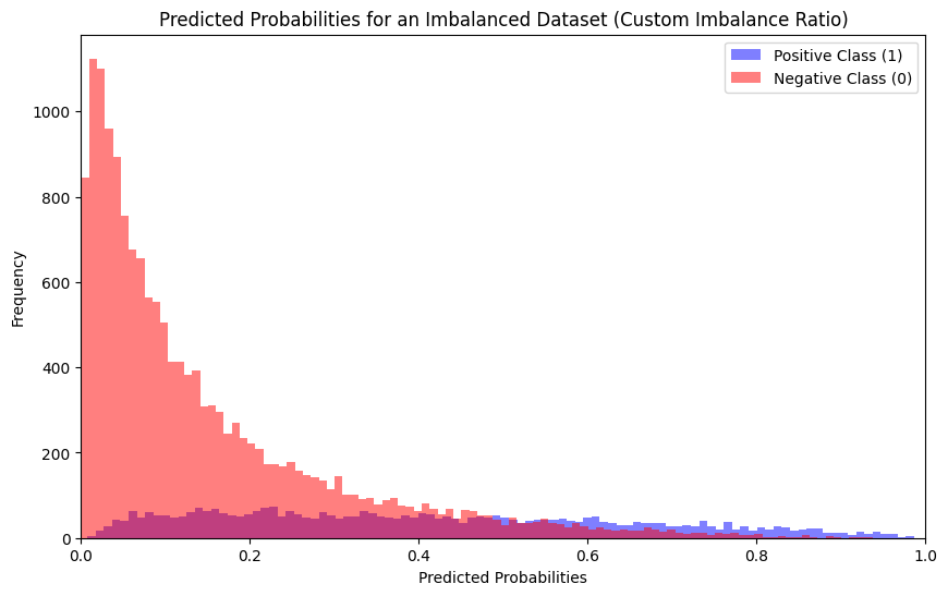
The histograms show the distribution of predicted probabilities for the positive and negative classes in an imbalanced dataset. The blue histogram shows the distribution of predicted probabilities for the positive class, and the red histogram shows the distribution of predicted probabilities for the negative class.
As can be seen, the positive class is much smaller than the negative class. This is because the dataset is imbalanced. The positive class is the minority class, and the negative class is the majority class.
The distribution of predicted probabilities for the negative class is right-skewed. This means that most of the negative examples have predicted probabilities that are close to 0. This is also a good sign, because it means that the model is able to confidently identify negative examples.
Threshold Optimization
The default threshold is often set to 0.5, but is it the best choice for our problem? To find out, we calculate several performance metrics, including the F1 score, recall, and precision, using the default threshold.
from sklearn.metrics import f1_score, recall_score, precision_score

# Calculate F1 score, recall, and precision for the default threshold (0.5)
default_threshold = 0.5
y_pred_default = (predicted_probabilities > default_threshold).astype(int)
f1_default = f1_score(y_test, y_pred_default)
recall_default = recall_score(y_test, y_pred_default)
precision_default = precision_score(y_test, y_pred_default)
Now comes the fun part. We experiment with different threshold values to see how they affect our model's performance. We calculate F1 scores, recall, and precision for a range of thresholds and plot the results.
# Vary the threshold and calculate F1 scores, recall, and precision
thresholds = np.linspace(0.1, 0.9, 18)
f1_scores = []
recall_scores = []
precision_scores = []

for threshold in thresholds:
    y_pred = (predicted_probabilities > threshold).astype(int)
    f1 = f1_score(y_test, y_pred)
    recall = recall_score(y_test, y_pred)
    precision = precision_score(y_test, y_pred)
    f1_scores.append(f1)
    recall_scores.append(recall)
    precision_scores.append(precision)
Visualizing the Results
The results are best presented visually. We create a plot that shows how the F1 score, recall, and precision change as we vary the decision threshold. We also include horizontal lines to indicate the performance metrics at the default threshold, making it easy to compare.
# Plot F1 scores, recall, and precision for different thresholds
plt.figure(figsize=(12, 6))
plt.plot(thresholds, f1_scores, marker='o', linestyle='-', label='F1 Score')
plt.plot(thresholds, recall_scores, marker='o', linestyle='-', label='Recall')
plt.plot(thresholds, precision_scores, marker='o', linestyle='-', label='Precision')
plt.axhline(f1_default, color='red', linestyle='--', label=f'F1 @ 0.5 Threshold: {f1_default:.2f}', alpha=0.7)
plt.axhline(recall_default, color='green', linestyle='--', label=f'Recall @ 0.5 Threshold: {recall_default:.2f}', alpha=0.7)
plt.axhline(precision_default, color='blue', linestyle='--', label=f'Precision @ 0.5 Threshold: {precision_default:.2f}', alpha=0.7)
plt.xlabel('Threshold')
plt.ylabel('Score')
plt.legend(loc='best')
plt.title('F1 Score, Recall, and Precision vs. Probability Threshold')
plt.grid()
plt.show()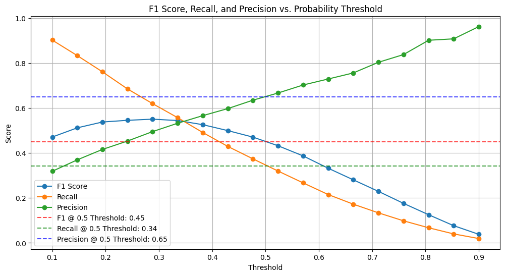
The plot shows that the F1 score, recall, and precision all vary as the threshold is changed. In general, as the threshold is lowered, the recall increases and the precision decreases. This is because a lower threshold will result in more positive predictions, which will increase the recall but also increase the number of false positives.
The optimal threshold is the value that maximizes the F1 score. In this plot, the optimal threshold appears to be around 0.3. At this threshold, the F1 score is approximately 0.55.
The dashed lines show the values of the F1 score, recall, and precision at the default threshold of 0.5. As can be seen, the F1 score, and recall are lower at the default threshold than they are at the optimal threshold.
Conclusion
Fine-tuning the decision threshold for your classifier can make a big difference in its performance, helping you customize the model to better fit the specific needs of your problem.
Next time you're working on a binary classification task, especially if you're dealing with an imbalanced dataset, take some time to play around with the decision threshold. You might be pleasantly surprised by how much it can boost your model's accuracy and usefulness.
Feel free to modify the code shared in this article and adapt it to your own datasets and models. By experimenting with these adjustments, you'll be able to get the most out of your classifiers.