
Insurance Price Optimization Walkthrough
Utilizing Generalized Linear Models and Non-Linear Programming to Maximize Profits

Introduction
In the insurance industry, setting the right price is crucial for achieving profitability and competitiveness. A price set too high may drive away customers, while a price set too low can lead to underwriting losses. The optimal price maximizes profitability by carefully considering the relationship between price, customer demand, and expected claim costs.
This article provides a comprehensive, step-by-step guide on how to build an insurance price optimization model. We will demonstrate how to:
Model customer demand and price elasticity using Generalized Linear Models (GLMs), accounting for how different customer segments react to price changes.
Model expected claim costs by separately modeling claim frequency and severity, a standard and robust actuarial technique.
Define distinct customer segments to allow for targeted pricing strategies.
Use Non-Linear Programming (NLP) to find the profit-maximizing price for each segment.
Step 1: Demand Modeling and Price Elasticity
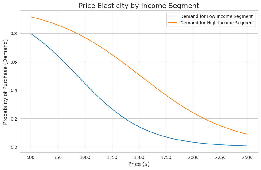
The first step is to understand how customers respond to price. The demand function estimates the probability that a customer will purchase a policy at a given price. We can model this using a logistic regression, but to make it more realistic, we will include an interaction term between price and income. This allows our model to learn that price sensitivity can differ across income levels.
First, we generate synthetic data and fit a Logit model.
import pandas as pd
import numpy as np
import statsmodels.api as sm
import matplotlib.pyplot as plt
import seaborn as sns
from scipy.optimize import minimize
from scipy.stats import logistic

# Set a consistent style for plots
sns.set_style("whitegrid")

def create_demand_data(n_samples=10000, random_seed=42):
    """
    Creates a sample dataset for demand modeling.
    Crucially, it includes an interaction term between price and income
    to model varying price elasticity.
    """
    np.random.seed(random_seed)

    # Feature Generation
    income = np.random.lognormal(mean=np.log(60000), sigma=0.5, size=n_samples)
    marketing_spend = np.random.uniform(50, 500, n_samples)
    price = np.random.uniform(500, 2500, n_samples)

    # The 'true' underlying model for purchase probability (log-odds)
    # A negative price coefficient means demand drops as price rises.
    # A positive income coefficient means higher income customers are more likely to buy.
    # The interaction term (price * income) is key: the negative effect of price
    # is dampened for customers with higher incomes.
    log_odds = (
        -0.5                         # Intercept
        - 4.0 * (price / 1000)       # Base price effect
        + 1.5 * (income / 100000)    # Income effect
        + 1.0 * (marketing_spend / 100) # Marketing effect
        + 2.0 * (price / 1000) * (income / 100000) # Interaction Term!
    )

    probability = logistic.cdf(log_odds)
    purchase = np.random.binomial(1, probability)

    df = pd.DataFrame({
        'income': income,
        'marketing_spend': marketing_spend,
        'price': price,
        'purchase': purchase
    })
    return df

def plot_demand_curves(demand_model_results, original_data):
    """
    Plots predicted demand curves for different income segments.
    """
    plt.figure(figsize=(10, 6))

    # Define income segments based on quantiles
    low_income = original_data['income'].quantile(0.25)
    high_income = original_data['income'].quantile(0.75)

    # Generate a range of prices to plot against
    price_range = np.linspace(
        original_data['price'].min(), original_data['price'].max(), 200
    )

    # Assume average marketing spend
    avg_marketing = original_data['marketing_spend'].mean()

    # Get the exact column names used by the demand model for training
    demand_exog_names = demand_model_results.model.exog_names

    for income_level, label in [(low_income, 'Low Income'), (high_income, 'High Income')]:
        # Create a raw DataFrame for prediction features
        plot_df_raw = pd.DataFrame({
            'price': price_range,
            'income': income_level,
            'marketing_spend': avg_marketing,
        })
        plot_df_raw['price_income_interaction'] = plot_df_raw['price'] * plot_df_raw['income']

        # Add constant and then reorder columns to match the model's exog_names
        # This is the crucial part to ensure 'const' is present and order is correct.
        plot_df_with_const = sm.add_constant(plot_df_raw, has_constant='add')

        # Select and reorder columns to match the trained model's exog_names
        # This handles cases where original features might not be in the same order
        # as exog_names after add_constant, or if some features were dropped.
        plot_df_ordered = plot_df_with_const[demand_exog_names]

        # Predict the probability of purchase
        pred_probs = demand_model_results.predict(plot_df_ordered)
        plt.plot(price_range, pred_probs, label=f'Demand for {label} Segment')

    plt.title('Price Elasticity by Income Segment', fontsize=16)
    plt.xlabel('Price ($)', fontsize=12)
    plt.ylabel('Probability of Purchase (Demand)', fontsize=12)
    plt.legend()
    plt.grid(True)
    plt.show()

def create_cost_data(n_samples=10000, random_seed=42):
    """
    Generates synthetic data for cost modeling.
    Claim frequency and severity are explicitly linked to features.
    """
    np.random.seed(random_seed)

    # Feature Generation
    driver_age = np.random.randint(18, 70, n_samples)
    vehicle_value = np.random.lognormal(mean=np.log(25000), sigma=0.6, size=n_samples)

    # --- Frequency Model (Poisson) ---
    # Younger drivers have higher claim frequency
    # Higher vehicle value is slightly correlated with more careful driving (lower freq)
    freq_log_lambda = (
        -1.5
        - 0.03 * (driver_age - 18)  # Negative correlation with age
        + 0.5 * np.log1p(vehicle_value / 10000) # Slight positive correlation
    )
    freq_lambda = np.exp(freq_log_lambda)
    number_of_claims = np.random.poisson(freq_lambda)

    # --- Severity Model (Gamma) ---
    # Higher vehicle value leads to much higher claim severity
    sev_log_mu = (
        6.0
        + 1.2 * np.log1p(vehicle_value / 10000) # Strong positive correlation
    )
    sev_mu = np.exp(sev_log_mu)
    # Gamma distribution shape parameter (controls variance)
    gamma_shape = 2.0
    claim_severity = np.random.gamma(shape=gamma_shape, scale=sev_mu / gamma_shape, size=n_samples)

    df = pd.DataFrame({
        'driver_age': driver_age,
        'vehicle_value': vehicle_value,
        'number_of_claims': number_of_claims,
        # Only observe severity if there was at least one claim
        'claim_severity': np.where(number_of_claims > 0, claim_severity, 0)
    })
    df['total_claim_amount'] = df['number_of_claims'] * df['claim_severity']
    return df

def plot_predicted_vs_actual_cost(freq_model_results, sev_model_results, df_cost):
    """
    Plots the predicted vs. actual total claim amount to assess cost model performance.
    """
    # Ensure consistency in feature names for prediction
    cost_features_for_prediction = ['driver_age', 'vehicle_value']

    # Create the raw prediction DataFrame
    X_test_raw = df_cost[cost_features_for_prediction].copy()

    # Add constant and then reorder columns for frequency model prediction
    X_freq_test_with_const = sm.add_constant(X_test_raw, has_constant='add')
    X_freq_test_ordered = X_freq_test_with_const[freq_model_results.model.exog_names]

    # Add constant and then reorder columns for severity model prediction
    X_sev_test_with_const = sm.add_constant(X_test_raw, has_constant='add')
    X_sev_test_ordered = X_sev_test_with_const[sev_model_results.model.exog_names]

    # Get predictions from both models
    predicted_freq = freq_model_results.predict(X_freq_test_ordered)
    predicted_sev = sev_model_results.predict(X_sev_test_ordered)
    df_cost['predicted_cost'] = predicted_freq * predicted_sev

    plt.figure(figsize=(10, 6))

    # Use a log scale due to the skewed nature of insurance costs
    plt.scatter(
        np.log1p(df_cost['total_claim_amount']),
        np.log1p(df_cost['predicted_cost']),
        alpha=0.3,
        label='Individual Policies'
    )

    # Add a reference line
    min_val = min(plt.xlim()[0], plt.ylim()[0])
    max_val = max(plt.xlim()[1], plt.ylim()[1])
    plt.plot([min_val, max_val], [min_val, max_val], 'r--', label='Perfect Prediction')

    plt.title('Cost Model Performance: Predicted vs. Actual Cost (Log Scale)', fontsize=16)
    plt.xlabel('Log(1 + Actual Total Claim Amount)', fontsize=12)
    plt.ylabel('Log(1 + Predicted Total Claim Amount)', fontsize=12)
    plt.legend()
    plt.show()

def optimize_price_for_segment(segment_features, demand_model_results, freq_model_results, sev_model_results):
    """
    Finds the optimal price for a customer segment using non-linear optimization.
    """
    # 1. Predict the cost for this segment
    cost_features_raw = pd.DataFrame([segment_features])

    # Prepare features for frequency model prediction
    freq_cost_features_with_const = sm.add_constant(cost_features_raw[['driver_age', 'vehicle_value']], has_constant='add')
    freq_cost_features_ordered = freq_cost_features_with_const[freq_model_results.model.exog_names]
    predicted_freq = freq_model_results.predict(freq_cost_features_ordered).iloc[0]

    # Prepare features for severity model prediction
    sev_cost_features_with_const = sm.add_constant(cost_features_raw[['driver_age', 'vehicle_value']], has_constant='add')
    sev_cost_features_ordered = sev_cost_features_with_const[sev_model_results.model.exog_names]
    predicted_sev = sev_model_results.predict(sev_cost_features_ordered).iloc[0]

    predicted_cost = predicted_freq * predicted_sev

    # 2. Define the negative profit function to be minimized
    def negative_profit(price):
        price = price[0] # scipy optimizer passes price as an array

        # Prepare raw features for demand prediction
        demand_features_raw = pd.DataFrame([{
            'price': price,
            'income': segment_features['income'],
            'marketing_spend': segment_features['marketing_spend']
        }])
        demand_features_raw['price_income_interaction'] = demand_features_raw['price'] * demand_features_raw['income']

        # Add constant and reorder columns to match the demand model's exog_names
        demand_features_with_const = sm.add_constant(demand_features_raw, has_constant='add')
        demand_features_ordered = demand_features_with_const[demand_model_results.model.exog_names]

        # Predict demand at the given price
        demand = demand_model_results.predict(demand_features_ordered).iloc[0]

        # Calculate profit and return its negative
        profit = (price - predicted_cost) * demand
        return -profit

    # 3. Run the optimization
    # Initial guess for the price and bounds
    initial_price_guess = [1500]
    # Price must be above cost, with a reasonable upper limit.
    # Add a small epsilon to predicted_cost to ensure it's strictly greater
    bounds = [(predicted_cost + 0.01, 5000)]

    result = minimize(negative_profit, initial_price_guess, method='SLSQP', bounds=bounds)

    optimal_price = result.x[0]
    max_profit = -result.fun

    return optimal_price, max_profit, predicted_cost

def plot_profit_curves(segments, results_df, demand_model_results, freq_model_results, sev_model_results):
    """
    Visualizes the profit curve for each segment, highlighting the optimal price.
    """
    plt.figure(figsize=(12, 7))

    # Get the exact column names used by the demand model
    demand_exog_names = demand_model_results.model.exog_names

    for idx, row in results_df.iterrows():
        segment_name = row['Segment']
        segment_features = segments[segment_name]
        predicted_cost = row['Predicted Cost']
        optimal_price = row['Optimal Price']

        # Generate a range of prices around the optimum
        price_range = np.linspace(predicted_cost + 0.01, optimal_price * 2, 300) # Ensure price > cost
        profits = []

        for price in price_range:
            # Prepare raw features for demand prediction
            demand_features_raw = pd.DataFrame([{
                'price': price, 'income': segment_features['income'],
                'marketing_spend': segment_features['marketing_spend']
            }])
            demand_features_raw['price_income_interaction'] = demand_features_raw['price'] * demand_features_raw['income']

            # Add constant and reorder columns to match the demand model's exog_names
            demand_features_with_const = sm.add_constant(demand_features_raw, has_constant='add')
            demand_features_ordered = demand_features_with_const[demand_exog_names]

            demand = demand_model_results.predict(demand_features_ordered).iloc[0]
            profit = (price - predicted_cost) * demand
            profits.append(profit)

        # Plot the curve
        plt.plot(price_range, profits, label=f'Profit Curve for: {segment_name}')
        # Mark the maximum
        plt.axvline(x=optimal_price, linestyle='--',
                    color=plt.gca().lines[-1].get_color(),
                    label=f'Optimal Price: ${optimal_price:,.2f}')

    plt.title('Profit Optimization Curves by Customer Segment', fontsize=16)
    plt.xlabel('Price ($)', fontsize=12)
    plt.ylabel('Expected Profit per Policyholder ($)', fontsize=12)
    plt.legend()
    plt.grid(True)
    plt.show()

def main():
    # Step 1: Demand Modeling and Price Elasticity
    df_demand = create_demand_data()
    X_demand_raw = df_demand[['price', 'income', 'marketing_spend']].copy()
    X_demand_raw['price_income_interaction'] = X_demand_raw['price'] * X_demand_raw['income']
    X_demand = sm.add_constant(X_demand_raw, has_constant='add') # Add constant here for training

    # Store the model object first, then fit it
    demand_model = sm.Logit(df_demand['purchase'], X_demand)
    demand_model_results = demand_model.fit(disp=False) # disp=False to suppress optimization messages
    print("--- Demand Model Results ---")
    print(demand_model_results.summary())
    plot_demand_curves(demand_model_results, df_demand)

    # Step 2: Cost Modeling (Frequency-Severity)
    df_cost = create_cost_data()
    features = ['driver_age', 'vehicle_value']

    # Fit Frequency Model
    X_freq = sm.add_constant(df_cost[features], has_constant='add') # Add constant here for training
    freq_model = sm.GLM(df_cost['number_of_claims'], X_freq, family=sm.families.Poisson())
    freq_model_results = freq_model.fit(disp=False)
    print("\n--- Frequency Model (Poisson GLM) Results ---")
    print(freq_model_results.summary())

    # Fit Severity Model (only on policies with claims)
    df_sev = df_cost[df_cost['number_of_claims'] > 0].copy()
    X_sev = sm.add_constant(df_sev[features], has_constant='add') # Add constant here for training
    sev_model = sm.GLM(df_sev['claim_severity'], X_sev, family=sm.families.Gamma(link=sm.families.links.log()))
    sev_model_results = sev_model.fit(disp=False)
    print("\n--- Severity Model (Gamma GLM) Results ---")
    print(sev_model_results.summary())
    plot_predicted_vs_actual_cost(freq_model_results, sev_model_results, df_cost)

    # Step 3: Defining Customer Segments
    customer_segments = {
        "Young Driver, Standard Car": {
            "driver_age": 22,
            "vehicle_value": 18000,
            "income": 45000,
            "marketing_spend": 150
        },
        "Experienced Driver, Economy Car": {
            "driver_age": 45,
            "vehicle_value": 12000,
            "income": 70000,
            "marketing_spend": 250
        },
        "Family Driver, High-Value SUV": {
            "driver_age": 40,
            "vehicle_value": 45000,
            "income": 110000,
            "marketing_spend": 300
        }
    }

    # Step 4: Non-Linear Price Optimization
    results = []
    for name, features in customer_segments.items():
        opt_price, max_prof, pred_cost = optimize_price_for_segment(
            features, demand_model_results, freq_model_results, sev_model_results
        )
        results.append({
            'Segment': name,
            'Predicted Cost': pred_cost,
            'Optimal Price': opt_price,
            'Max Profit per Policyholder': max_prof
        })

    results_df = pd.DataFrame(results)
    print("\n--- Price Optimization Results ---")
    print(results_df.round(2))

    # Step 5: Results and Visualization
    plot_profit_curves(customer_segments, results_df, demand_model_results, freq_model_results, sev_model_results)

if __name__ == "__main__":
    main()
The interaction between price and income is visualized in the plot below. The demand curve for the "High Income Segment" is both higher and flatter than for the "Low Income Segment". This shows that higher-income customers are not only more likely to purchase a policy overall, but their decision is also less affected by price increases i.e. they have lower price elasticity.
Step 2: Cost Modeling (Frequency-Severity)
Next, we model the expected cost per policy. A robust method is to model two components separately:
Claim Frequency: The number of claims a policyholder makes. Modeled with a Poisson GLM.
Claim Severity: The average cost of each claim. Modeled with a Gamma GLM.
The total expected cost is then Expected Frequency * Expected Severity.
Frequency Model 🚗
The Poisson GLM results show the coefficient for driver_age is negative, confirming that claim frequency tends to decrease as a driver gets older.
--- Frequency Model (Poisson GLM) Results ---
                 Generalized Linear Model Regression Results
==============================================================================
Dep. Variable:       number_of_claims   No. Observations:                10000
Model:                            GLM   Df Residuals:                     9997
Model Family:                 Poisson   Df Model:                            2
Link Function:                    Log   Scale:                          1.0000
Method:                          IRLS   Log-Likelihood:                -5515.5
Date:                Sun, 25 May 2025   Deviance:                       6943.8
Time:                        18:45:31   Pearson chi2:                 9.89e+03
No. Iterations:                     6   Pseudo R-squ. (CS):            0.04898
Covariance Type:            nonrobust
=================================================================================
                    coef    std err          z      P>|z|      [0.025      0.975]
---------------------------------------------------------------------------------
const            -0.6484      0.067     -9.714      0.000      -0.779      -0.518
driver_age       -0.0288      0.002    -19.173      0.000      -0.032      -0.026
vehicle_value  9.587e-06   8.31e-07     11.539      0.000    7.96e-06    1.12e-05
=================================================================================
Severity Model 💰
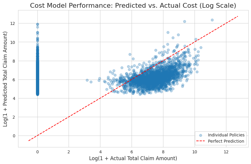
The performance of our combined cost model is visualized in the scatter plot below showing predicted vs. actual claim costs on a log scale, with points clustering around a 45-degree line, indicating good model performance. The wide scatter is expected for insurance data, and the dense vertical line at x=0 represents the many policies with no claims.
Step 3: Defining Customer Segments
With our models built, we define specific customer segments to find a tailored price for each.
# We define three distinct customer segments
customer_segments = {
    "Young Driver, Standard Car": {
        "driver_age": 22,
        "vehicle_value": 18000,
        "income": 45000,
        "marketing_spend": 150
    },
    "Experienced Driver, Economy Car": {
        "driver_age": 45,
        "vehicle_value": 12000,
        "income": 70000,
        "marketing_spend": 250
    },
    "Family Driver, High-Value SUV": {
        "driver_age": 40,
        "vehicle_value": 45000,
        "income": 110000,
        "marketing_spend": 300
    }
}
Step 4: Non-Linear Price Optimization
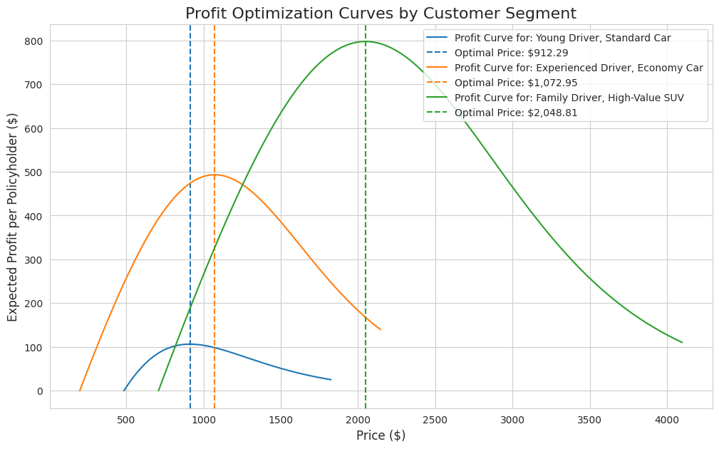
For each segment, we define a profit function: Profit(Price) = (Price - Predicted_Cost) * Demand(Price). Because the demand component is non-linear, we use a Non-Linear Programming (NLP) solver (scipy.optimize.minimize) to find the price that maximizes this function.
The results are summarized in the table below. The model has successfully identified a unique optimal price and expected profit for each distinct customer segment.
Young Driver, Standard Car:
Predicted Cost: $485.61
Optimal Price: $912.29
Max Profit per Policyholder: $106.34
Experienced Driver, Economy Car:
Predicted Cost: $199.57
Optimal Price: $1,072.95
Max Profit per Policyholder: $493.17
Family Driver, High-Value SUV:
Predicted Cost: $708.94
Optimal Price: $2,048.81
Max Profit per Policyholder: $797.50
Step 5: Results and Visualization
The final plot illustrates our solution with each curve representing the expected profit for a segment across a range of prices. The optimizer has found the peak of each curve, marked by the dashed line. This visualization shows the profit-maximizing price for the "Family Driver" is more than double that of the "Young Driver", ultimately, demonstrating why a one-price-fits-all strategy is suboptimal.
Sources:
https://scikit-learn.org/stable/auto_examples/linear_model/plot_tweedie_regression_insurance_claims.html
https://web.actuaries.ie/sites/default/files/erm-resources/Emphasis2010_1_art4_Price_Opt.pdf